In many cases of analysis of algorithms, we encounter the hypergeometric distribution, which is basically sampling without replacement. There are unfortunately a lot of different notations used, as is nicely summed up in Matthew Skala’s survey. I will not be making the situation better, as for this post I’ll use another notation still:
| Chvátal | MathWorld | Wikipedia | This post | |
|---|---|---|---|---|
| Balls in urn | N | n+m | N | n |
| Balls that count | M | n | K | pn |
| Balls that don’t count | N-M | m | N-K | (1-p)n |
| Balls you draw | n | N | n | sn |
We usually approximate the sampling as sampling with replacement, thereby getting the binomial distribution. Thus it comes as no surprise, that we can bound the tail of the hypergeometric just like the tail of the binomial. This has a sleek proof by Chvátal or simply using anti correlation and Hoefding.
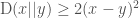
![\begin{aligned} \Pr[X\ge(p+t)s n] &\le \exp(-s n \text{D}(p+t||p))\\ &\le \exp(-2t^2sn) \end{aligned}](https://s0.wp.com/latex.php?latex=%5Cbegin%7Baligned%7D+%5CPr%5BX%5Cge%28p%2Bt%29s+n%5D+%26%5Cle+%5Cexp%28-s+n+%5Ctext%7BD%7D%28p%2Bt%7C%7Cp%29%29%5C%5C+%26%5Cle+%5Cexp%28-2t%5E2sn%29+%5Cend%7Baligned%7D&bg=ffffff&fg=444444&s=0&c=20201002)
Here 
However, while the binomial is only a good approximation to the hypergeometric, when the fraction of sampled elements $latex s$ is small. I’ve often wondered how much better we could actually do, when the number of sampled balls is close to the total number. The answer is as follows:
![\begin{aligned} \Pr[X\le(p-t)s n] &\le \exp(-sn\text{D}(p-t||p)) &\le \exp(-2t^2sn)\\ \Pr[X\le(p-t)s n] &\le \exp(-(1-s)n\text{D}(p+\tfrac{ts}{1-s}||p)) &\le \exp(-\tfrac{s}{1-s}2t^2sn)\\ \Pr[X\ge(p+t)s n] &\le \exp(-sn\text{D}(p+t||p)) &\le \exp(-2t^2sn)\\ \Pr[X\ge(p+t)s n] &\le \exp(-(1-s)n\text{D}(p-\tfrac{ts}{1-s}||p)) &\le \exp(-\tfrac{s}{1-s}2t^2sn)\\ \end{aligned}](https://s0.wp.com/latex.php?latex=%5Cbegin%7Baligned%7D+%5CPr%5BX%5Cle%28p-t%29s+n%5D+%26%5Cle+%5Cexp%28-sn%5Ctext%7BD%7D%28p-t%7C%7Cp%29%29+%26%5Cle+%5Cexp%28-2t%5E2sn%29%5C%5C+%5CPr%5BX%5Cle%28p-t%29s+n%5D+%26%5Cle+%5Cexp%28-%281-s%29n%5Ctext%7BD%7D%28p%2B%5Ctfrac%7Bts%7D%7B1-s%7D%7C%7Cp%29%29+%26%5Cle+%5Cexp%28-%5Ctfrac%7Bs%7D%7B1-s%7D2t%5E2sn%29%5C%5C+%5CPr%5BX%5Cge%28p%2Bt%29s+n%5D+%26%5Cle+%5Cexp%28-sn%5Ctext%7BD%7D%28p%2Bt%7C%7Cp%29%29+%26%5Cle+%5Cexp%28-2t%5E2sn%29%5C%5C+%5CPr%5BX%5Cge%28p%2Bt%29s+n%5D+%26%5Cle+%5Cexp%28-%281-s%29n%5Ctext%7BD%7D%28p-%5Ctfrac%7Bts%7D%7B1-s%7D%7C%7Cp%29%29+%26%5Cle+%5Cexp%28-%5Ctfrac%7Bs%7D%7B1-s%7D2t%5E2sn%29%5C%5C+%5Cend%7Baligned%7D&bg=ffffff&fg=444444&s=0&c=20201002)
While the two ‘elegant’ versions of the bounds, in the third column, are somewhat weaker than the entropy bounds, they make the difference stand out clearly: For the hypergeometric distribution it is possible to add a factor 


We can show the above bounds by making use of symmetry to swap 

Let 
![H_{-}(M,N,n,k) = \Pr[X\le k]](https://s0.wp.com/latex.php?latex=H_%7B-%7D%28M%2CN%2Cn%2Ck%29+%3D+%5CPr%5BX%5Cle+k%5D&bg=ffffff&fg=444444&s=0&c=20201002)
![H_{+}(M,N,n,k) = \Pr[X\ge k]](https://s0.wp.com/latex.php?latex=H_%7B%2B%7D%28M%2CN%2Cn%2Ck%29+%3D+%5CPr%5BX%5Cge+k%5D&bg=ffffff&fg=444444&s=0&c=20201002)
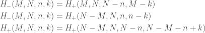
The arguments are mostly similar, so we’ll just do bound number two:
![\begin{aligned} \Pr[X\le(p-t)s n] &= H_{-}(pn,n,sn,(p-t)sn)\\ &= H_{+}(pn,n,n-sn,pn-(p-t)sn)\\ &= H_{+}(pn,n,(1-s)n,(p+\tfrac{ts}{1-s})(1-s)n)\\ &\le \exp(-(1-s)n\text{D}(p+\tfrac{ts}{1-s}||p)) \end{aligned}](https://s0.wp.com/latex.php?latex=%5Cbegin%7Baligned%7D+%5CPr%5BX%5Cle%28p-t%29s+n%5D+%26%3D+H_%7B-%7D%28pn%2Cn%2Csn%2C%28p-t%29sn%29%5C%5C+%26%3D+H_%7B%2B%7D%28pn%2Cn%2Cn-sn%2Cpn-%28p-t%29sn%29%5C%5C+%26%3D+H_%7B%2B%7D%28pn%2Cn%2C%281-s%29n%2C%28p%2B%5Ctfrac%7Bts%7D%7B1-s%7D%29%281-s%29n%29%5C%5C+%26%5Cle+%5Cexp%28-%281-s%29n%5Ctext%7BD%7D%28p%2B%5Ctfrac%7Bts%7D%7B1-s%7D%7C%7Cp%29%29+%5Cend%7Baligned%7D&bg=ffffff&fg=444444&s=0&c=20201002)
Another way we might have gone around finding the bounds, would be studying Stirling approximation of the main term 

